Free Fall Simulator & 1D Motion Virtual Lab
📎 Embed this Virtual Lab
Are you an educator, science communicator, or webmaster?
You can easily embed this simulation directly into your class website, LMS (Canvas, Google Classroom), or blog.
We only ask for two simple things:
- ✅ Credit the source: AulaQuest.com
- 🚫 Non-commercial use only
Copy the code below:
<iframe src="https://aulaquest.com/s/fisica/caida-libre/index.php"
  width="100%"
  height="560"
  style="border: 1px solid #ccc; border-radius: 8px;"
  allowfullscreen
title="Advanced Free Fall Simulator - AulaQuest"></iframe>1. Core Principle: The Physics of Free Fall
Ideal free fall is the one-dimensional motion of an object subject only to the influence of gravity. In a perfect vacuum (where Air Resistance is set to "Zero"), gravity pulls downwards with a constant acceleration, meaning the object's velocity increases at a steady rate.
In the real world, objects falling through an atmosphere experience a second force: Air Resistance (Drag). While gravity pulls the object down, drag pushes it back up. The faster the object falls, the stronger the drag becomes, eventually leading to a state where the object stops accelerating entirely.
2. Key Equations & Mathematical Model
When studying free fall in a vacuum, we use the standard kinematic equations for uniform acceleration. You can verify these formulas in real-time using the simulator's data table:
- $v_f$ = Final velocity ($m/s$ or $ft/s$)
- $v_0$ = Initial velocity ($m/s$ or $ft/s$)
- $g$ = Acceleration due to gravity ($9.8\ m/s^2$ or $32.2\ ft/s^2$)
- $t$ = Time elapsed ($s$)
- $\Delta y$ = Displacement / Change in vertical position ($m$ or $ft$)
3. Essential Vocabulary
The constant, maximum speed that a freely falling object eventually reaches when the resistance of the medium (drag) prevents further acceleration.
A dimensionless number used to quantify the drag or resistance of an object in a fluid environment, such as air or water. A lower $C_d$ means the object is more aerodynamic.
The overall vector sum of all the forces acting on an object. In free fall with air resistance, it is the difference between the downward force of gravity and the upward drag force.
A graphical illustration used to visualize the applied forces, movements, and resulting reactions on a body in a given condition. (Toggle "Show Vectors" in the simulator to see a live FBD).
4. Graphical Analysis: Interpreting Kinematic Curves
Visualize the mathematical behavior of falling objects in real-time:
- Position (y-t): A parabolic curve. It clearly shows how displacement increases quadratically over time.
- Velocity (v-t): A straight diagonal line. The slope directly represents the acceleration due to gravity ($g$).
- Acceleration (a-t): A constant horizontal line (e.g., $9.8 \text{ m/s}^2$ or $32.2 \text{ ft/s}^2$).
5. Advanced Physics: Linear vs. Quadratic Drag
In the real world, air resistance isn't one-size-fits-all. Aulaquest's physics engine calculates vector forces frame-by-frame using two distinct mathematical models based on your class level:
Typical for very small objects (like fog droplets) or highly viscous fluids (like oil).
Drag force is directly proportional to velocity. Terminal velocity ($v_t$) is reached when Weight ($mg$) equals Drag ($kv$).
The standard for free fall in air at high speeds (skydivers, baseballs, rockets).
Drag force is proportional to the square of the velocity. It acts much more aggressively at higher speeds.
💡 Note on the "Air Resistance" Slider
The percentage you select (e.g., 10%) acts as a scaling factor. We engineered it with high sensitivity so students can observe terminal velocity over short, manageable distances (e.g., 100m / 300ft). In Earth's atmosphere, it would require thousands of feet of free fall to collect the same data!
Free Fall & 1D Kinematics
Rigorous exploration of 1D motion, data linearization, and real-world fluid dynamics.
Instructor Notes & Lesson Overview
This virtual lab is specifically aligned with standard US curricula:
- AP Physics 1: Kinematics (1D Motion, Free-Body Diagrams, Terminal Velocity).
- NGSS: HS-PS2-1 (Motion and Stability: Forces and Interactions).
- SWBAT analyze position vs. time and velocity vs. time graphs for accelerating objects.
- SWBAT calculate the experimental value of $g$ using linearized data.
- SWBAT differentiate between constant acceleration (vacuum) and decreasing acceleration (drag).
Addressing Common Misconceptions
Misconception: Heavier objects naturally fall faster than lighter objects.
Correction: Assign the "Apollo 15 Challenge" (Tab 3) or use the Dual Drop mode with 0% Air Resistance to visually prove that mass is independent of acceleration in a vacuum.
Misconception: Acceleration stops when an object is falling fast.
Correction: Toggle "Show Vectors" to demonstrate how the upward drag vector eventually matches the downward gravity vector, resulting in a Net Force of zero (Terminal Velocity).
Suggested 45-Minute Lesson Flow
1. Pre-Lab (10 min): Introduce the concept of free fall. Ask students to predict the shape of a position vs. time graph for a dropped object.
2. In-Lab Inquiry (25 min): Have students load a specific Teacher Preset URL. Instruct them to pause the simulator every 0.4 seconds to collect data points and complete the "Calculating 'g'" activity (Tab 2) in their lab notebooks.
3. Post-Lab Assessment (10 min): Use Aulaquest's built-in Quick Theory and Self-Grading Quiz features to verify student understanding and instantly review the class statistics.
Experimental Deduction of Gravity
Data linearization is a fundamental scientific technique that allows us to extract universal physical constants from non-linear natural behaviors. In this experiment, students will transform a parabolic free-fall curve into a linear relationship to determine the experimental value of $g$.
Mathematical Foundation
The position of an object in free fall follows the standard kinematic model for uniform acceleration:
If dropped from rest ($v_{0y} = 0$), the displacement $\Delta y = |y - y_0|$ is simply:
We compare this physical model with the slope-intercept form of a linear equation ($Y = m \cdot X + b$):
- Y-variable: Displacement ($\Delta y$).
- X-variable: Time squared ($t^2$).
- Y-intercept $b$: $0$ (Starts from rest).
- Slope $m$: Equivalent to $\frac{1}{2}g$.
- Result: $g = 2 \cdot m$
Experimental Data Logging
To verify this relationship, students must perform systematic data collection using the simulation's measurement tools. Important Note: The values presented in the table below are an illustrative approximation. Encourage your students to collect their own raw data from the virtual lab.
| $t$ (s) | $t^2$ ($s^2$) | $y$ (m | ft) | $\Delta y$ (m | ft) | $g_{exp} = 2\Delta y/t^2$ |
|---|---|---|---|---|
| 0.40 | 0.16 | 199.22 m (653.6 ft) | 0.78 m (2.56 ft) | 9.75 m/s² (32.0 ft/s²) |
| 0.80 | 0.64 | 196.86 m (645.8 ft) | 3.14 m (10.3 ft) | 9.81 m/s² (32.2 ft/s²) |
| 1.20 | 1.44 | 192.94 m (633.0 ft) | 7.06 m (23.1 ft) | 9.80 m/s² (32.1 ft/s²) |
| 1.60 | 2.56 | 187.45 m (614.9 ft) | 12.55 m (41.1 ft) | 9.81 m/s² (32.2 ft/s²) |
| 2.00 | 4.00 | 180.39 m (591.8 ft) | 19.61 m (64.3 ft) | 9.81 m/s² (32.2 ft/s²) |
Reality: Position vs. Time
Analysis: Displacement vs. $t^2$
Analysis Conclusions
- Linearity: Graphing displacement against time squared yields a straight line, confirming that acceleration is constant.
- Accuracy: The calculated value of $g$ should approximate $9.81 \text{ m/s}^2$ ($32.2 \text{ ft/s}^2$). Small deviations are excellent discussion points for measurement uncertainty.
- Physical Interpretation: The slope of the line does not represent gravity directly, but rather half of it ($m = g/2$).
Critical Thinking Labs
- Activate Dual Mode to compare two simultaneous drops.
- Select Object A: Bowling Ball (5 kg / 11 lbs).
- Select Object B: Feather (10 g / 0.02 lbs).
- Key Condition: Set Air Resistance to 0% (ideal vacuum).
- Drop both objects from 100 m (328 ft) and observe the position-time graph.
- Do two distinct curves appear? No. The trajectories overlap completely. Nature confirms Galileo: Mass does not matter in a vacuum.
1. Relationship between velocity and time
Starting from rest, the velocity equation is: $$ v_f = g\,t $$ Solving for time ($t$): $$ t = \frac{v_f}{g} = \frac{14.88}{3.72} = \mathbf{4.00\ \text{s}} $$
2. Calculating the drop height
Using the kinematic position equation: $$ h = \frac{1}{2}\,g\,t^2 $$ Substituting values: $$ h = \frac{1}{2}\cdot 3.72 \cdot (4.00)^2 = \mathbf{29.76\ \text{m}}\ (97.6\ \text{ft}) $$
Select the Mars environment, adjust the initial height to $h \approx 29.8\ \text{m} \ (97.8\ \text{ft})$ and verify with the chronometer that the impact occurs exactly at $t = 4.0\ \text{s}.$
Your Challenge: Interplanetary Comparison
Calculate how much longer the feather takes to fall on the Moon compared to Earth, dropped from an astronaut's shoulder height ($1.6\text{m} / 5.2\text{ft}$).
$t = \sqrt{2h/g} = \sqrt{3.2/9.8}$
$t \approx \mathbf{0.57 \text{ s}}$
$t = \sqrt{2h/g} = \sqrt{3.2/1.62}$
$t \approx \mathbf{1.40 \text{ s}}$
Fluid Dynamics: AulaQuest's Physics Engine
AulaQuest utilizes a numerical resolution engine that calculates vector forces frame-by-frame. This allows for analyzing the complete dynamics of a fall: how drag force increases with velocity, how acceleration progressively decreases, and why it ultimately reaches zero when dynamic equilibrium is achieved.
Pedagogical use of the "% Air Resistance" slider
The drag slider does not represent a real physical coefficient of the air. It is a dimensionless control parameter. It is engineered with high sensitivity so that terminal velocity is observable over manageable laboratory distances (10 m – 500 m).
Physical Properties of Objects
| Object | Mass ($m$) | Radius ($r$) | Drag Coef. $C_d$ |
|---|---|---|---|
| Cannonball | 50 kg (110 lbs) | 12 cm (4.7 in) | 0.47 |
| Bowling Ball | 5 kg (11 lbs) | 18 cm (7.1 in) | 0.47 |
| Astronaut | 100 kg (220 lbs) | 40 cm (15.7 in) | 1.00 |
| Soccer Ball | 0.45 kg (1.0 lb) | 18 cm (7.1 in) | 0.25 |
| Ping Pong Ball | 2.7 g (0.006 lbs) | 2 cm (0.8 in) | 0.50 |
| Feather | 10 g (0.02 lbs) | 10 cm (3.9 in) | 2.00 |
Drag force is directly proportional to velocity. Typical of highly viscous fluids or very small scale objects (Stokes' Drag).
Drag force is proportional to the square of velocity. The standard model for free fall in air (Newton's Drag).
🔍 Verification Guide: Earth ($g = 9.81 m/s^2$) & 6% Air Resistance. Quadratic Model.
Calculated vt: 10.75 m/s (35.3 ft/s)
Calculated vt: 36.07 m/s (118.3 ft/s)
Velocity vs. Time Graph Behavior
Your Classroom. Your Conditions. Your Method.
Configure the simulation with your initial values, hide controls, and lock variables. Students won't just "explore randomly": they enter the precise physical scenario you've designed.
- URL Access linked directly to your teacher configuration
- Variables locked for deep calculation and reasoning tasks
- Integrated self-grading activities sent directly to your dashboard
No quick answers here. Students formulate hypotheses, record raw data, build tables, analyze graphs, and write comprehensive conclusions. A complete lab experience with real scientific rigor.
- Manual section-by-section grading, just like a traditional lab report
- Individual and group progress tracking from the Teacher Dashboard
- Direct grading and PDF report generation
Available exclusively for Verified Educators.